
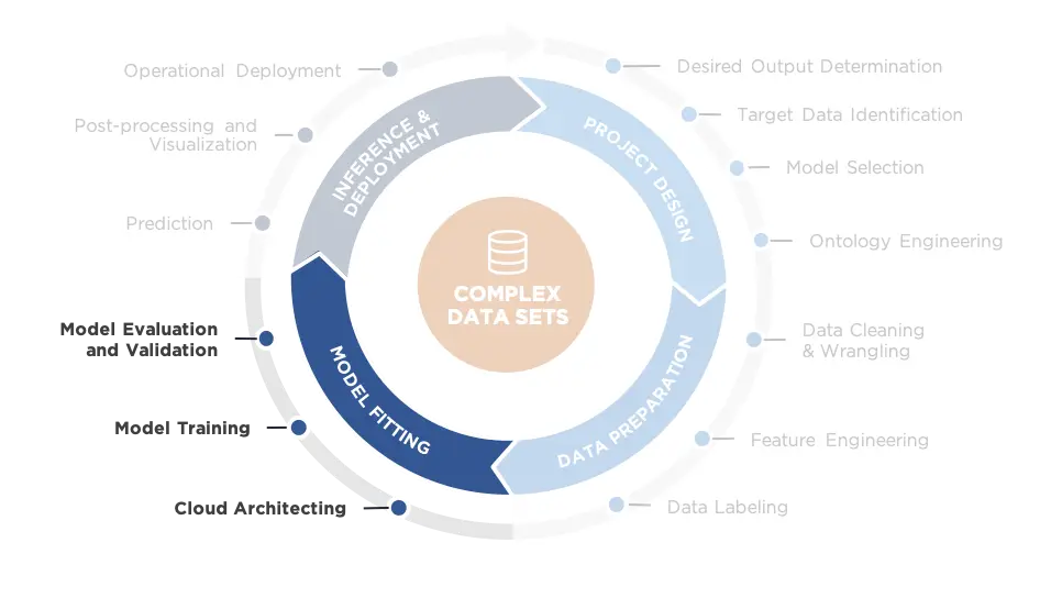
Even though the bulk of the work happens during the data preparation and labeling phase in quadrant two, model fitting constitutes the meat and potatoes of Machine Learning (ML). This third phase of the ML Lifecycle is iterative and slow—a full training run may take days or even weeks.
Early versions of the model are likely to perform poorly, so meaningful benchmarks should be put in place early in the process to assess the performance of the model. Adding layers to a neural network architecture necessarily increases model complexity and requires fitting new parameters. That, in turn, requires more training data to make up for degrees of freedom that are consumed by the new parameters. Adding layers without good reason is as likely to hurt training performance as it is to help.
To speed iteration, it’s important to terminate a model early if it is not performing well and possibly revisit the training ontology. “Performing well” for an ML model means it is beginning to converge. Early on, model convergence is the single most meaningful indicator of promising model performance—even more so than accuracy. Because model training and validation occur simultaneously and increase in tandem, you ideally want to observe the training and validation losses decreasing in tandem as well. This gradual process is known as model convergence. Train until such time as the validation accuracy or loss plateaus. If validation accuracy begins to plateau as training accuracy continues to rise, this signifies overfitting. At this point, the model is simply learning the training data, not the inherent patterns and dependencies within.
Step One: Cloud Architecting
Phase three in the ML Lifecycle begins with ensuring you have the right compute environment for model training, either on-premise or in a public cloud platform. (Some organizations also maintain private cloud platforms.) GCP, AWS, and Azure all offer data science-ready cloud platforms. GPU-enabled cloud compute for neural network training is expensive; your cost optimization may point to buying hardware rather than renting it from a commercial cloud computing provider. Once owned, you can reuse the same hardware for many projects.
Whether hardware is rented from a commercial cloud provider or purchased, leveraging the compute resources fully and avoiding unnecessary costs takes designing a storage and compute environment comprised of physical or virtual machines capable of running distributed training, validation, and testing cycles at various throughput. If you opt for a cloud environment, architects will need to spin up virtual machines with appropriate specifications (i.e., number of CPU cores, memory, or number and type of GPUs) to achieve the desired training speed at an acceptable price point. They also must ensure that the model code has been optimized to fully utilize the cluster. For example, utilize multiple GPUs by loading the entire model on each GPU and dividing the training data into batches that are individually allocated to a GPU. This strategy requires parameters to be stored centrally and continuously updated as each GPU processes a batch.
An alternative strategy is to break up the model into parts. Each resides on a separate machine and all data passes through this model cascade. Not all models can be decomposed in a manner that allows this, but for those that can, we have found it to be more efficient.
Determining Your need for cloud compute
NT Concepts utilizes cloud compute providers for model training. The approach enables us to construct a training environment on demand. Our environments consist of the latest generation of GPU hardware at whatever scale is most efficient for the particular training job. We typically work on up to four large models at any given time, in addition to small-scale sandboxing. We generally lack the flexibility to sequence our training to deconflict use of compute resources, so we benefit from the ability to spin up a single compute cluster designed especially for a bespoke training job. The secondary benefits are that we do not have to maintain hardware, do not incur costs for hardware upgrades, and have an easy time attributing compute costs to specific jobs.
To determine whether or not cloud compute makes sense for you depends on how much network training you do and what your ability is to sequence it. The hardware requirements for a job depend on the size of the network being trained as well as the nature and amount of the training data. Textual data can be divided into smaller batches than data consisting of high-resolution multi-channel images. Some neural network architectures may be able to derive greater benefit from parallel computing than others.
Once the compute environment is in place for a given project, the slow and iterative processes of model training and model evaluation and validation can begin.
Step Two: Model Training
Deep Learning models are specified through their network architecture (addressed in model selection), hyperparameters, and finally through the choice of data features to serve as predictors.
Hyperparameters are parameters that cannot be optimized through the normal stochastic gradient descent procedures, as well as variations on neural network architecture. Systematic ways exist to optimize or “tune” hyperparameters, though the effort can be computationally burdensome because they typically involve brute force optimization rather than a guided optimization procedure. These include a gridded search through the hyperparameter “space”, as well as randomly generating hyperparameter sets according to some probability distribution. Validation of a model tuning should make use of a separate reserved dataset that is distinct from both the training and test sets.
The process of choosing data features may involve the raw data exactly as it was wrangled and labeled, as well as additional features derived by transforming the raw features. This process is known as feature engineering. As an example, if the raw data contains geographic points, engineered features may include the distances between those points. The process of feature engineering to improve model performance is more of an art than a science. On the one hand, engineered features that are linked alongside raw features consume degrees of freedom, so that process must be done sparingly. On the other hand, engineered features used in place of raw features limit what a model is capable of learning.
Many of the decisions made in previous phases, like ontology design, are subject to revision during the model training phase. With rare exceptions like the Network Architecture Search algorithm, the only reliable way to search this space for model versions that perform well is to iteratively test nearly limitless variations against benchmarks. Measuring progress in model improvement demands the project have a meaningful benchmark that reflects a real application and a test of how well an existing model performs a task (not some commonly used heuristic of performance).
For example, while custom-tailoring a natural language processing model for a client to extract and classify entities in a corpus of chatroom text (commonly called “named entity recognition”), the natural benchmarks are the “F1” score. That score measures the tradeoff of false extractions and missed extractions, and the rate of correct classification given correct extraction. The benchmark that actually matters, however, is the time it takes a human overseeing the model to obtain a result with the model as compared to without (the baseline). Even if heuristics are well aligned, they are not the same.
Data engineers break the labeled images into training, testing, and tuning subsets, and use the training subset to initially fit the selected models. To fully train and become minimally viable, a model needs to complete a large number of full model iterations through the training data. This process takes time. (Investing in beefy GPUs can help, like Nvidia’s Tesla V100, but the process of revision and iteration remains tedious.)
A real-world example of model training: neural networks
Training a neural network is the practice of passing training data into the neural network and optimizing the network parameters to minimize the difference between the predictions and the correct output (the “loss”). As with other model training processes, optimization is iterative. If the network trains, the data team can expect the loss trend to decrease from iteration to iteration, reaching a minimum once the model has converged. It is normal for the loss to increase in individual training “steps,” however, since any given batch of data passed into the model may not be well predicted by the current set of parameters. Predictions should get more accurate until they reach a plateau. Be aware that an algorithm may not train, due to the particulars of the network structure. It’s the procedures for batching data and passing those batches through the network iteratively, along with the optimization algorithm, that may determine success.
Because it can take a substantial amount of time to fully train a large network, it is important to monitor loss and accuracy. This focus allows the team to detect training failures and kill the training job quickly and then shift the focus to identifying opportunities for model improvement. The TensorFlow framework includes a lightweight application called TensorBoard that is very useful for this purpose, provided you first generate and log the loss and accuracy.
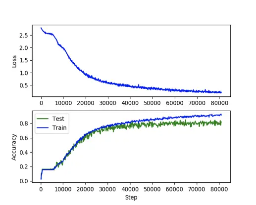
The top graph shows a reduction in loss over the course of many training iterations. The bottom graph is the improvement of prediction (validation) accuracy against the training and test sets. The loss never strictly decreases and accuracy never strictly increases, making it difficult to automate the detection of training failure in this scenario. Signs of training failure include loss that blows up or accuracy that craters. Instances in which model training leads to changes in loss but that do not form any clear increasing or decreasing trend can be tougher to spot.
With regard to managing parameters and hyperparameters, NT Concepts’ general practice is to employ the simplest possible network requiring the fewest number of parameters to accomplish the objective. It is not always feasible to augment those data through field tests or new intelligence collection and analysis. We employ models that make the most of the limited data.
It’s worthwhile to reiterate that every extra parameter in a model consumes a degree of freedom. If two models function identically but the first model has fewer parameters than the second, the former may outperform the latter, especially when the labeled dataset is small. The tradeoff in this scenario is whether the additional predictive power offered by a new network layer will make up for the loss of accuracy resulting from the consumption of degrees of freedom. In the face of inconsistent outcomes, err on the side of model simplicity.
Models with fewer layers will have fewer hyperparameters to tune and fewer structural variations to test, which will reduce the amount of iteration needed. Toward this end, NT Concepts’ team of scientists engages best practices like sizing convolution layers to correspond to the actual resolution of images being analyzed rather than applying unnecessary padding, which would require fitting parameters that correspond to neurons not being used.
Keep in mind that early versions of a model are likely to perform poorly. This preliminary, poorly-performing model that shows signs of convergence is known as a Minimum Viable Model (MVM). It generally will be untuned. Establish a meaningful benchmark against which to recognize poor training before it becomes a liability. Designing an efficient training architecture is important to the outcome.
Step Three: Model Evaluation and Validation
The final step in quadrant three is to verify and validate the model. Verification is the process of ensuring a model is internally consistent with itself. (If inconsistencies are seen, they usually come from different operations performed when the model is training to fit the parameters—not when the model is predicting using the particular set of parameters.) Validating the model ensures that predictions meet desired accuracy thresholds against a previously unused dataset (called the tuning set or validation set). The tuning set assesses model performance and tunes the models’ hyperparameters, cross-validating to ensure robustness, and diagnosing possible over-fitting.
With verification and validation, the data science team can quantify the final model’s performance and highlight false positive and false negative detection rates. With the phase complete, the team can leverage the model to make viable predictions, post-process the results, and visualize them.
We will explore the processes and hidden challenges in the Inference and Deployment phase of the ML Lifecycle phase in our next post in this series.